Question

Two-point charges $\mathop q\nolimits_A = 3\mu C$ and $\mathop q\nolimits_B = - 3\mu C$ are located 20 cm apart in vacuum.
(a) What is the electric field at the midpoint O of the line AB joining the two charges?
(b) If a negative test charge of magnitude $\mathop {1.5 \times 10}\nolimits^{ - 9} C$ is placed at this point, what is the force experienced by the test charge?

Answer 1

(i) Electric field due to a given charge in the space around the charge can be defined as the electrostatic force of attraction or repulsion experienced by any other charge in the space due to the given charge.
(ii) The electric field intensity at any point is the strength of the electric field at that point. It is defined as the force experienced by a unit test charge placed at that point within the field of the other charge.
i.e. $\vec E\left( {\vec r} \right) = \dfrac{{\vec F\left( {\vec r} \right)}}{{{q_0}}}$(1)
Where $\vec F\left( {\vec r} \right) =$Force acting on the test charge, ${q_0} =$Test charge, and $\vec E\left( {\vec r} \right) =$ Electric field intensity

Complete step by step answer:
(a) Step 1: As given in the problem two-point charges $\mathop q\nolimits_A = 3\mu C$, $\mathop q\nolimits_B = - 3\mu C$and distance between these two-point charges i.e. $r = 20$cm. Another point $O$ at the mid of line joining these two-point charges, taken and an electric field is to be calculated at this point O.

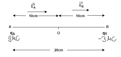
The total electric field at this point O will be the sum of the electric fields due to point charges $\mathop q\nolimits_A$ i.e. $\overrightarrow {\mathop E\nolimits_A }$ and $\mathop q\nolimits_B$ i.e. $\overrightarrow {\mathop E\nolimits_B }$ respectively.
So, the magnitude of net electric field at point O is-
$E = \mathop E\nolimits_A + \mathop E\nolimits_B$ (2)
Electric field at point O caused by $\mathop q\nolimits_A$ charge,
$\mathop E\nolimits_A = \dfrac{1}{{4\pi {\varepsilon _0}}}\dfrac{{\mathop q\nolimits_A }}{{^{\mathop r\nolimits_A^2 }}}$ direction along OB (3)
Where ${\varepsilon _0} =$Permittivity of free space, $\mathop r\nolimits_A =$ Distance of point O from $\mathop q\nolimits_A$
Similarly, Electric field at point O caused by $\mathop q\nolimits_B$ charge,
$\mathop E\nolimits_B = \dfrac{1}{{4\pi {\varepsilon _0}}}\dfrac{{\mathop q\nolimits_B }}{{^{\mathop r\nolimits_B^2 }}}$ direction along OB (4)
Where ${\varepsilon _0} =$ Permittivity of free space, $\mathop r\nolimits_B =$Distance of point O from $\mathop q\nolimits_B$

Step 2: Now from putting the values from equations (3) and (4) into equation (2), we get-
$E = \dfrac{1}{{4\pi {\varepsilon _0}}}\dfrac{{\mathop q\nolimits_A }}{{^{\mathop r\nolimits_A^2 }}} + \dfrac{1}{{4\pi {\varepsilon _0}}}\dfrac{{\mathop q\nolimits_B }}{{^{\mathop r\nolimits_B^2 }}}$ (5)
Where $\mathop r\nolimits_A = 10$cm, $\mathop r\nolimits_B = 10$cm, and $\dfrac{1}{{4\pi {\varepsilon _0}}} = 9 \times \mathop {10}\nolimits^9$ $Nm^2C^{-2}$
After keeping all the values in equation (5), we will get-
$E = 9 \times \mathop {10}\nolimits^9 \times \dfrac{{3 \times \mathop {10}\nolimits^{ - 6} }}{{\left( {\mathop {10 \times 10}\nolimits^{ - 2} } \right) \times \left( {\mathop {10 \times 10}\nolimits^{ - 2} } \right)}} + 9 \times \mathop {10}\nolimits^9 \times \dfrac{{3 \times \mathop {10}\nolimits^{ - 6} }}{{\left( {\mathop {10 \times 10}\nolimits^{ - 2} } \right) \times \left( {\mathop {10 \times 10}\nolimits^{ - 2} } \right)}}$N/C
$E = 2 \times 9 \times \mathop {10}\nolimits^9 \times \dfrac{{3 \times \mathop {10}\nolimits^{ - 6} }}{{\left( {\mathop {10 \times 10}\nolimits^{ - 2} } \right) \times \left( {\mathop {10 \times 10}\nolimits^{ - 2} } \right)}}$ N/C
$E = 54 \times \mathop {10}\nolimits^5$N/C along OB.
So, the electric field at the mid-point is $E = 5.4 \times \mathop {10}\nolimits^6$N/C along $OB$.

(b) Step 1: A test charge of amount $\mathop { - 1.5 \times 10}\nolimits^{ - 9}$C is placed at mid-point. Let’s say this charge is $\mathop q\nolimits_C$.
So, $\mathop {\mathop q\nolimits_C = - 1.5 \times 10}\nolimits^{ - 9}$C. Here negative sign will help while deciding the direction of force.
The force experienced by this charge $= F$and can be calculated by-
$F = \mathop q\nolimits_C E$
$F = \mathop {1.5 \times 10}\nolimits^{ - 9} \times 5.4 \times \mathop {10}\nolimits^6$N
$F = 8.1 \times \mathop {10}\nolimits^{ - 3}$N along OA.
The magnitude of the force is $F = 8.1 \times \mathop {10}\nolimits^{ - 3}$N and the direction of the force on the test charge are along with $OA$ because the force on the charge at $O$ will be attractive in nature due to charge on $A$ and repulsive in nature due to $B$. So, the direction will be along with $OA$.

$\therefore$ The total angular width of central maxima in this diffraction pattern is $2\theta = 5 \times \mathop {10}\nolimits^{ - 2}$radian.

Note:
(i) Electric field $\overrightarrow E$ due to source charge $Q$ does not depend upon test charge $\mathop q\nolimits_0$. This is because $\overrightarrow F \mathop { \propto q}\nolimits_0$, so that the ratio $\dfrac{{\overrightarrow F }}{{\mathop q\nolimits_0 }}$ does not depend on $\mathop q\nolimits_0$.
(ii) From the knowledge of electric field intensity $\overrightarrow E$at any point $\overrightarrow r$, we can readily calculate the magnitude and direction of force experienced by any charge $\mathop q\nolimits_0$ held at that point, i.e., $\overrightarrow F \mathop {(\overrightarrow r ) = q}\nolimits_0 \overrightarrow E (\overrightarrow r )$