Question
Question: The plot of $\frac{1}{\Lambda_m}$ against $c\Lambda_m$ for aqueous solution of weak monobasic acid (...
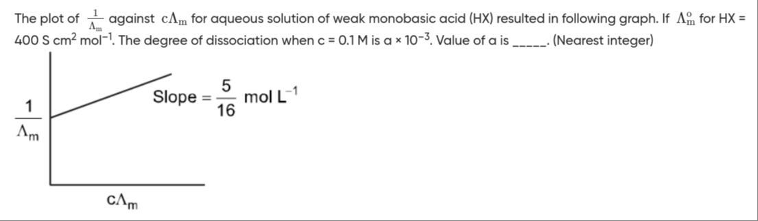
The plot of Λm1 against cΛm for aqueous solution of weak monobasic acid (HX) resulted in following graph. If Λm∘ for HX = 400 S cm2 mol−1. The degree of dissociation when c = 0.1 M is a × 10−3. Value of a is _______. (Nearest integer)
14
Solution
The relationship between molar conductivity (Λm), limiting molar conductivity (Λm∘), concentration (c), and degree of dissociation (α) for a weak electrolyte is given by Ostwald's Dilution Law.
-
Ostwald's Dilution Law:
For a weak monobasic acid HX, the dissociation equilibrium is:
HX⇌H++X−
The dissociation constant Ka is given by:
Ka=[HX][H+][X−]=1−αcα2 -
Relation between α and Λm:
The degree of dissociation α is also related to molar conductivities:
α=Λm∘Λm -
Deriving the linear relationship:
Substitute α from the second equation into the first equation:
Ka=1−Λm∘Λmc(Λm∘Λm)2
Ka=(Λm∘)2(Λm∘Λm∘−Λm)cΛm2
Ka=Λm∘(Λm∘−Λm)cΛm2Rearrange the equation to match the given plot of Λm1 vs cΛm:
KaΛm∘(Λm∘−Λm)=cΛm2
Divide both sides by Λm:
KaΛm∘(ΛmΛm∘−1)=cΛm
Divide both sides by KaΛm∘:
ΛmΛm∘−1=KaΛm∘cΛm
ΛmΛm∘=1+KaΛm∘cΛm
Divide both sides by Λm∘:
Λm1=Λm∘1+Ka(Λm∘)2cΛmThis equation is in the form y=mx+b, where:
y=Λm1
x=cΛm
Slope (m) =Ka(Λm∘)21
Y-intercept (b) =Λm∘1 -
Calculate Ka:
Given:
Slope =165 mol L−1
Λm∘=400 S cm2 mol−1We need to ensure consistent units. The slope is given in mol L−1, which is equivalent to mol dm−3.
Λm∘ is in S cm2 mol−1. To make units consistent, we can convert Λm∘ to S dm2 mol−1 or convert the slope.
Let's use Λm∘ in S cm2 mol−1 and ensure Ka units are consistent.
Ka typically has units of mol L−1 (or M).
The term Ka(Λm∘)2 will have units of (mol L−1) (S cm2 mol−1)2 = mol L−1 S2 cm4 mol−2 = S2 cm4 L−1 mol−1.
Therefore, the slope Ka(Λm∘)21 should have units of S−2 cm−4 L mol.
However, the given slope is in mol L−1. This implies that the equation used in the graph implicitly assumes a certain unit conversion factor or that the units for the slope are specific to the graph's context.
Let's assume the given slope value directly corresponds to Ka(Λm∘)21 without further unit conversions for the numerical value, or that the Ka value will be obtained in units consistent with the slope.
The most common form of Ostwald's dilution law for Ka is Ka=1−αcα2, where c is in mol/L and Ka is in mol/L.
The equation Λm1=Λm∘1+Ka(Λm∘)2cΛm is often used with Λm in S cm2 mol−1, c in mol L−1 and Ka in mol L−1.
In this case, the units of Ka(Λm∘)21 would be (mol L−1)(S cm2mol−1)21=mol S2cm4L. This is not mol L−1.Let's re-examine the units of the slope given. If the slope is 1/(Ka(Λm∘)2), and the units of Ka are mol/L, and Λm∘ are S cm2 mol−1, the units of the slope should be mol S2cm4L.
However, if c is expressed in M (mol/L) and Λm in S cm2 mol−1, then cΛm has units of M S cm2 mol−1 = (mol/L) S cm2 mol−1 = S cm2 L−1.
And 1/Λm has units of S−1 cm−2 mol.
So, the slope Δ(cΛm)Δ(1/Λm) would have units of S cm2L−1S−1cm−2mol=S−2cm−4mol L.
The given slope is 165 mol L−1. This unit implies that some conversion factor for volume (cm3 to L) is absorbed or the units are simplified for Ka.Let's assume the given slope value is numerically correct for the expression Ka(Λm∘)21 and we need to determine Ka.
Slope =Ka(Λm∘)21
165=Ka(400)21
Ka=5×(400)216=5×16000016=80000016=500001
Ka=2×10⁻⁵ mol L−1 (or M) -
Calculate degree of dissociation (α) when c=0.1 M:
We use the formula Ka=1−αcα2.
Given c=0.1 M and Ka=2×10⁻⁵ M.
Since the acid is weak, α is usually very small, so we can approximate 1−α≈1.
Ka≈cα2
2×10−5=0.1×α2
α2=0.12×10−5=2×10⁻⁴
α=2×10−4=2×10⁻²
α≈1.414×10⁻²Let's check the approximation. If α=1.414×10−2=0.01414, then 1−α=0.98586, which is close to 1. So the approximation is valid.
-
Express α in the required format:
α=1.414×10−2=14.14×10⁻³
The problem asks for α=a×10−3.
So, a=14.14. -
Nearest integer value of a:
The nearest integer to 14.14 is 14.
The final answer is 14.