Question

Point charges $+3.0\mu C$ and $+7.0\mu C$ are located at the origin and at the point (0.5m, 0) respectively in the x-y plane. Find the electric field at points:
A. (0.5m, 0.9m), B. (1.0m, 0) and C. (1.0m, -0.3m)

Answer 1

Recall the expression for electric field due to a point charge q. We are given the coordinates of the points at which the charges are kept as well as that of the point at which the electric field is to be found. From that we could find the magnitude of r and hence find electric fields due to each charge. Apply superposition principle to find the electric field due to the system.
Formula used:
Expression for electric field,
$E\left( r \right)=\dfrac{1}{4\pi {{\varepsilon }_{0}}}\dfrac{q}{{{r}^{2}}}\widehat{r}$

Complete answer:
In the question, we are given two point charges whose locations are also clearly given. Also we are given three points and we are asked to find the electric field at these points due to these charges.
We know that the electric field at a point at distance r from a point charge q is given by,
$E\left( r \right)=\dfrac{1}{4\pi {{\varepsilon }_{0}}}\dfrac{q}{{{r}^{2}}}\widehat{r}$
Where, r is the magnitude of the displacement vector connecting these points and $\widehat{r}$ gives the direction.
The electric field at point A due to the given charges:

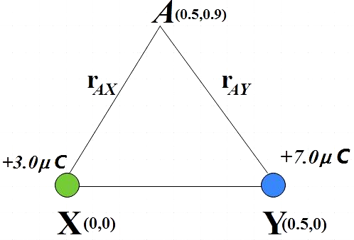
Electric field due to $+3.0\mu C$ at point A,
Magnitude of displacement vector = $\left| {{r}_{AX}} \right|$
$\left| {{r}_{AX}} \right|=\sqrt{{{\left( 0.5-0 \right)}^{2}}+{{\left( 0.9-0 \right)}^{2}}}=1.02m$
${{E}_{1}}=\dfrac{1}{4\pi {{\varepsilon }_{0}}}\dfrac{+3.0\times {{10}^{-6}}}{{{1.02}^{2}}}=9\times {{10}^{9}}\times \dfrac{3.0\times {{10}^{-6}}}{1.0404}$
$\Rightarrow {{E}_{1}}=25.95\times {{10}^{3}}N{{C}^{-1}}$ ……………………….. (1)
Electric field due to $+7.0\mu C$ at point A,
Magnitude of displacement vector = $\left| {{r}_{AY}} \right|$
$\left| {{r}_{AY}} \right|=\sqrt{{{\left( 0.5-0.5 \right)}^{2}}+{{\left( 0.9-0 \right)}^{2}}}=0.9m$
${{E}_{2}}=\dfrac{1}{4\pi {{\varepsilon }_{0}}}\dfrac{+7.0\times {{10}^{-6}}}{{{0.9}^{2}}}=9\times {{10}^{9}}\times \dfrac{7.0\times {{10}^{-6}}}{0.81}$
$\Rightarrow {{E}_{2}}=77.78\times {{10}^{3}}N{{C}^{-1}}$…………………………… (2)
From the superposition principle, the electric field at point A due to the given charges is given by the sum of (1) and (2),
$\Rightarrow {{E}_{A}}={{E}_{1}}+{{E}_{2}}$
$\Rightarrow {{E}_{A}}=\left( 25.95+77.78 \right)\times {{10}^{3}}N{{C}^{-1}}$
$\Rightarrow {{E}_{A}}=103.73\times {{10}^{3}}N{{C}^{-1}}$
The electric field at point B due to the given charges:

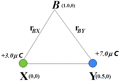
Electric field due to $+3.0\mu C$ at point B,
Magnitude of displacement vector = $\left| {{r}_{BX}} \right|$
$\left| {{r}_{BX}} \right|=\sqrt{{{\left( 1.0-0 \right)}^{2}}+{{\left( 0-0 \right)}^{2}}}=1.0m$
${{E}_{3}}=\dfrac{1}{4\pi {{\varepsilon }_{0}}}\dfrac{+3.0\times {{10}^{-6}}}{{{1}^{2}}}=9\times {{10}^{9}}\times 3.0\times {{10}^{-6}}$
$\Rightarrow {{E}_{3}}=27\times {{10}^{3}}N{{C}^{-1}}$ ……………………….. (3)
Electric field due to $+7.0\mu C$ at point B,
Magnitude of displacement vector = $\left| {{r}_{BY}} \right|$
$\left| {{r}_{BY}} \right|=\sqrt{{{\left( 1.0-0.5 \right)}^{2}}+{{\left( 0-0 \right)}^{2}}}=0.5m$
${{E}_{4}}=\dfrac{1}{4\pi {{\varepsilon }_{0}}}\dfrac{+7.0\times {{10}^{-6}}}{{{0.5}^{2}}}=9\times {{10}^{9}}\times \dfrac{7.0\times {{10}^{-6}}}{0.25}$
$\Rightarrow {{E}_{4}}=252\times {{10}^{3}}N{{C}^{-1}}$…………………………… (4)
From the superposition principle, the electric field at point B due to the given charges is given by the sum of (3) and (4),
$\Rightarrow {{E}_{B}}={{E}_{3}}+{{E}_{4}}$
$\Rightarrow {{E}_{B}}=\left( 27+252 \right)\times {{10}^{3}}N{{C}^{-1}}$
$\Rightarrow {{E}_{B}}=279\times {{10}^{3}}N{{C}^{-1}}$
The electric field at point C due to the given charges:

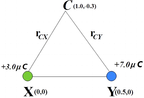
Electric field due to $+3.0\mu C$ at point C,
Magnitude of displacement vector = $\left| {{r}_{CX}} \right|$
$\left| {{r}_{CX}} \right|=\sqrt{{{\left( 1.0-0 \right)}^{2}}+{{\left( -0.3-0 \right)}^{2}}}=1.04m$
${{E}_{5}}=\dfrac{1}{4\pi {{\varepsilon }_{0}}}\dfrac{+3.0\times {{10}^{-6}}}{{{1.04}^{2}}}=9\times {{10}^{9}}\times \dfrac{3.0\times {{10}^{-6}}}{1.09}$
$\Rightarrow {{E}_{5}}=24.77\times {{10}^{3}}N{{C}^{-1}}$ ……………………….. (5)
Electric field due to $+7.0\mu C$ at point C,
Magnitude of displacement vector = $\left| {{r}_{CY}} \right|$
$\left| {{r}_{CY}} \right|=\sqrt{{{\left( 1.0-0.5 \right)}^{2}}+{{\left( -0.3-0 \right)}^{2}}}=0.58m$
${{E}_{6}}=\dfrac{1}{4\pi {{\varepsilon }_{0}}}\dfrac{+7.0\times {{10}^{-6}}}{{{0.58}^{2}}}=9\times {{10}^{9}}\times \dfrac{7.0\times {{10}^{-6}}}{0.34}$
$\Rightarrow {{E}_{6}}=185.29\times {{10}^{3}}N{{C}^{-1}}$…………………………… (6)
From the superposition principle, the electric field at point C due to the given charges is given by the sum of (5) and (6),
$\Rightarrow {{E}_{C}}={{E}_{5}}+{{E}_{6}}$
$\Rightarrow {{E}_{C}}=\left( 24.77+185.29 \right)\times {{10}^{3}}N{{C}^{-1}}$
$\Rightarrow {{E}_{C}}=210.06\times {{10}^{3}}N{{C}^{-1}}$
Therefore, the electric field at points A, B and C are respectively given by,
$\Rightarrow {{E}_{A}}=103.73\times {{10}^{3}}N{{C}^{-1}}$
$\Rightarrow {{E}_{B}}=279\times {{10}^{3}}N{{C}^{-1}}$
$\Rightarrow {{E}_{C}}=210.06\times {{10}^{3}}N{{C}^{-1}}$

Note:
Though we have represented all the three cases in figures, the actual location of the points may not necessarily be the corners of a triangle. So, keep this in mind that the figure is drawn for better understanding and doesn’t represent the exact location of the points. Since, both the point charges are positive, we know that the electric field lines will be directed radially outward.