Question
Question: In the figure, \(\epsilon = 12.0 V,\; R_1 = 2000\Omega,\; R_2 = 3000\Omega,\; R_3 = 4000\Omega\). Wh...
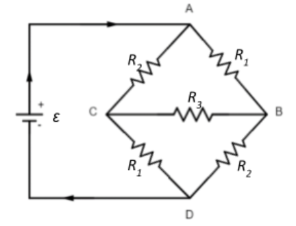
In the figure, ϵ=12.0V,R1=2000Ω,R2=3000Ω,R3=4000Ω. What are the potential differences (a) VA–VB (b) ) VB–VC (c) ) VC–VD and (d) ) VA–VC ?
Solution
In order to find the potential differences across the given terminals, we need to find the current flowing through the resistances across the terminals. For this, we need only two tools. At either node B or C apply Kirchhoff’s Current Law (KCL) to obtain current flowing through R3 in terms of current flowing through R1 and R2.
Then, apply Kirchhoff’s Voltage Law (KVL) to the two loops EACDE and EABCDE and obtain simultaneous expressions for the currents through R1 and R2 and solve to determine the numerical values of currents through the different resistances. To this end, use ohm’s law to determine the voltage drops across the resistances across the given terminals and arrive at the appropriate potential differences for the same.
Formula used: Kirchhoff’s Current Law (KCL): Ientering+Iexiting=0
Kirchhoff’s Voltage Law (KVL): ΣV=0
Ohm’s law: V=IR
Complete step by step answer:
Let us begin by deconstructing the circuit and analysing the current flow through it.
The current flows from the positive terminal to the negative terminal of the battery via the resistance setup across nodes A and D. At node A, the current splits up into two to flow through resistances R1 and R2. Let the current flowing through these resistances be i1 and i2 respectively.
Since the resistances seem to be following a symmetry in the way they are arranged, we can say that the current flowing through them can also be extrapolated under the same symmetry.
Since we have RAB=RCD=R1, we can say that the same current i1 flows through both the resistances. Similarly, since RAC=RBD=R2, we can say that the same current i2 flows through both the resistances.
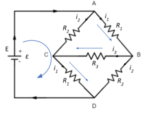
Now, at node B, the current again splits up into two branches to flow through R3 and R2. Let the current flowing through R3 be i3.
At the node B, we can apply Kirchhoff’s Current Law (KCL) which suggests that the algebraic sum of currents entering a node will be equal to the sum of currents leaving a node. From the diagram, we see that at node B, applying KCL gives us:
i1=i3+i2⇒i3=i1−i2. Thus, the current flowing through R3 is the difference between the currents flowing through R1 and R2.
Now, let us bring in Kirchhoff’s Voltage Law (KVL) which suggests that the sum of all voltages around any closed loop in a circuit must be equal to zero. Since our circuit consists of two independent closed loops, let us apply KVL and see how it goes from there.
Applying KVL in the external loop EACDE of our circuit we get:
ϵ−i2R2−i1R1=0
Given that ϵ=12V, R1=2kΩ, R2=3kΩ
⇒12–i2(3kΩ)−i1(2kΩ)=0
⇒2000i1+3000i2=12
Similarly, applying KVL to the loop EABCDE we get:
ϵ–i1R1−i3R3−i1R1=0
⇒ϵ−2i1R1–(i1−i2)R3=0
Given that R3=4kΩ
⇒12–2i1(2kΩ)−(i1−i2)(4kΩ)=0
⇒−8000i1+4000i2=−12⇒−2000i1+1000i2=−3
Solving the two KVL equations simultaneously we get:
4000i2=9⇒i2=40009
⇒i2=2.25mA
Substituting this is the first KVL equation we get:
2000i1+3000(2.25×10⁻³)=12⇒2000i1=12−6.75⇒i1=20005.25
⇒i1=2.625mA
Then, i3=i1−i2=2.625−2.25=0.375mA
Now that we have found the current through each resistance, we can now find the required potential differences which are nothing but the voltage drops across the resistances in the corresponding branches.
(a) VA–VB=i1R1=(2.625×10−3)×(2×103)=5.25V
(b) VB–VC=i3R3=(0.375×10−3)×(4×103)=1.5V
(c) VC–VD=i1R1=(2.625×10−3)×(2×103)=5.25V
(d) VA–VC=i2R2=(2.25×10−3)×(3×103)=6.75V
Note: Though we looked at KCL and KVL from a quantitative perspective, it is important to understand what they mean in a physical sense.
KCL signifies conservation of charge since the law basically suggests that the sum of currents entering a node must be equal to the sum of currents leaving the node, which means that electric charges are neither ambiguously lost nor mysteriously added but remains the same in an isolated system.
KVL signifies conservation of energy since the total energy in a system remains constant, though it may be transferred between components of the system in the form of electric potential and current.