Question

Find the electric field vector at ${{P}}\left( {{{a,a,a}}} \right)$ due to infinitely long lines of charges along ${{x,y}}$ and ${{z}}$ axes respectively. The charge density i.e. charge per unit length is ${{\lambda }}{{.}}$

Answer 1

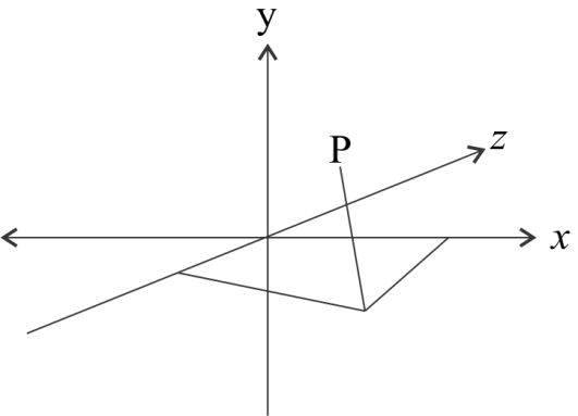
In This question, we have three line charges which will produce an electric field around them. To find the net magnitude of the electric field and its direction we will use superposition principle i.e. we first individually calculate the value of Electric field due to each line charge and then sum up to find the net Electric field.

Formula used:
The electric field due to line charge is given by (i) ${{E}}\;{{ = }}\,\dfrac{{{\lambda }}}{{{{2\pi }}{{{\varepsilon }}_{{0}}}}}{{.\hat r}}$
Where ‘E’ is electric field
$\lambda$ is linear charge density i.e. charge per unit length.
${\varepsilon _0}$ is permittivity of free space
$r$ is perpendicular distance from the line charge
$\hat r$ is unit vector in the direction of electric field.
(ii) ${{\hat r}}\;{{ = }}\;\dfrac{{{{\vec r}}}}{{\left| {{{\vec r}}} \right|}}$ where $\hat r$ is unit vector along $\vec r$, is position vector and $\left| {\vec r} \right|$ is magnitude of ${{\vec r}}{{.}}$

Complete step by step solution:
(i) Electric field due to line charge X-axis

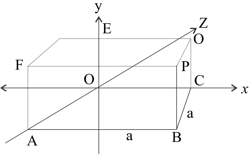
Here we have charge density of line charge is $\lambda ,$ and clear from the diagram that $CP$ is perpendicular distance of Point $P$ form line charge OX
Further from the triangle $BCP$ it is clear that, by Pythagoras theorem.
{{CP}}\;{{ = }}\;\sqrt {{{B}}{{{C}}^{{2}}}{{ + B}}{{{P}}^{{2}}}} \\_\\_\left( 1 \right)

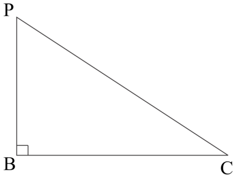
We have give BC$=$ PB$=$ a
So, substituting these values in $\left( 1 \right)$ we get
\left| {\overrightarrow {{{CP}}} } \right|\;{{ = }}\sqrt {{2}} {{a}}\;{{\\_\\_\\_}}\left( {{2}} \right)
We know, the electric field at any distance which is radially outward from line can be found by relation {{{F}}_{{x}}}{{ = }}\dfrac{{{\lambda }}}{{{{2\pi }}{{{\varepsilon }}_{{0}}}\left| {\overrightarrow {{{CP}}} } \right|}}{{.}}\widehat {{{CP}}}\;{{\\_\\_\\_}}\left( {{3}} \right)
Where $\widehat {{{CP}}}$ is unit vector along $\overrightarrow {{{CP}}}$
In vector form $\overrightarrow {{{CP}}} \;{{ = }}\;{{a\hat j + a\hat k}}$
So, \widehat {{{CP}}}{{ = }}\dfrac{{\overrightarrow {{{CP}}} }}{{\left| {\overrightarrow {{{CP}}} } \right|}}{{ = }}\;\dfrac{{{{a\hat j + a\hat k}}}}{{\sqrt {{2}} {{a}}}}{{ = }}\dfrac{{{{\hat j + \hat k}}}}{{\sqrt {{2}} }}\;{{\\_\\_}}\left( {{4}} \right)
Put the values from $\left( 2 \right)$ and $\left( 4 \right)$ in $\left( 3 \right)$ we get,
{{{E}}_{{x}}}{{ = }}\dfrac{{{\lambda }}}{{{{2\pi }}{{{\varepsilon }}_{{0}}}\sqrt {{2}} {{a}}}}{{.}}\dfrac{{\left( {{{\hat j + \hat k}}} \right)}}{{\sqrt {{2}} }}{{\\_\\_\\_}}\left( {{5}} \right)
(ii) Electric field due to line charge along Z axis in this case $\overrightarrow {{{AP}}}$ is perpendicular vector from line charge form Point ${{P}}{{.}}$ which can be obtained from triangle ${{BAP}}{{.}}$
In vector form $\overrightarrow {{{AP}}} {{ = a\hat i + a\hat j}}$ and magnitude of $\overrightarrow {{{AP}}}$ is given as,
$\left| \overrightarrow{{AP}} \right|\ {=}\ \sqrt{{A}{{{B}}^{{2}}}{+B}{{{P}}^{{2}}}}$
\left| \overrightarrow{{AP}} \right|\ {=}\ \sqrt{{2}}{.a}\ { }\\!\\!\\_\\!\\!{ }\\!\\!\\_\\!\\!{ }\\!\\!\\_\\!\\!{ }\left( {6} \right)
If $\widehat {{{AP}}}$ is unit vector along $\overrightarrow {{{AP}}\;}$ then,
\widehat {{{AP}}}\;{{ = }}\;\dfrac{{\overrightarrow {{{AP}}} }}{{\left| {\overrightarrow {{{AP}}} } \right|}}\;{{ = }}\;\dfrac{{{{a\hat i + a\hat j}}}}{{\sqrt {{2}} {{a}}}}\;{{ = }}\;\dfrac{{{{\hat i + \hat j}}}}{{\sqrt {{2}} }}\;{{\\_\\_\\_}}\left( {{7}} \right)
If ${{{E}}_{{z}}}$ represents electric field due to line charge along ${{y}}$ axis then,
{{{E}}_{{y}}}{{ = }}\;\dfrac{{{\lambda }}}{{{{2\pi }}{{{\varepsilon }}_{{0}}}\left| {\overrightarrow {{{AP}}} } \right|}}{{.}}\;\widehat {{{AP}}}\;{{\\_\\_\\_}}\left( {{8}} \right)
From equation $\left( 6 \right),\left( 7 \right)$ and $\left( 8 \right)$, we get ,
{{{E}}_{{z}}}{{ = }}\,\dfrac{{{\lambda }}}{{{{2\pi }}{{{\varepsilon }}_{{0}}}\sqrt {{2}} {{.a}}}}\;\dfrac{{\left( {{{\hat i + \hat j}}} \right)}}{{\sqrt {{2}} }}\;{{\\_\\_\\_}}\left( {{9}} \right)
(iii) electric field due to line charge along y-axis in this case $\overrightarrow {{{EP}}}$ is perpendicular vector from line charge to point ${{P,}}$ which can be obtained from triangle ${{FEP}}$
In vector form, $\overrightarrow {{{EP}}} \;{{ = }}\;{{a\hat i + a\hat j}}$
In magnitude form,
$\left| \overrightarrow{{EP}} \right|\ {=}\ \sqrt{{F}{{{P}}^{{2}}}{+E}{{{P}}^{{2}}}}$
\left| \overrightarrow{{EP}} \right|\ {=}\ \sqrt{{2}}{.a}\ { }\\!\\!\\_\\!\\!{ }\\!\\!\\_\\!\\!{ }\\!\\!\\_\\!\\!{ }\\!\\!\\_\\!\\!{ }\left( {10} \right)
Also unit vector along $\overrightarrow {{{EP}}}$ can be calculated as,
\widehat {{{EP}}}\;{{ = }}\;\dfrac{{\overrightarrow {{{EP}}} }}{{\left| {\overrightarrow {{{EP}}} } \right|}}\;{{ = }}\;\dfrac{{{{a\hat i + a\hat j}}}}{{\sqrt {{2}} {{.a}}}}\;{{ = }}\;\dfrac{{\left( {{{\hat i + \hat j}}} \right)}}{{\sqrt {{2}} }}\;{{\\_\\_}}\left( {{{11}}} \right)
So, if $\overrightarrow {{{{E}}_{{y}}}}$ gives the electric field due to line charge along ${{y}}$ axis then it is evaluated as,
{\overrightarrow {{E}} _{{y}}}\;{{ = }}\;\dfrac{{{\lambda }}}{{{{2\pi }}{{{\varepsilon }}_{{0}}}\left| {\overrightarrow {{{EP}}} } \right|}}{{.}}\;\widehat {{{EP}}}\;{{\\_\\_}}\left( {{{12}}} \right)
By equations $\left( {10} \right),\left( {11} \right)$ and $\left( {12} \right)$
{\overrightarrow {{E}} _{{y}}}\;{{ = }}\;\dfrac{{{\lambda }}}{{{{2\pi }}{{{\varepsilon }}_{{0}}}\sqrt {{2}} {{a}}}}\;\dfrac{{\left( {{{\hat i + \hat j}}} \right)}}{{\sqrt {{2}} }}\;{{\\_\\_\\_\\_}}\left( {{{13}}} \right)

After adding equation $\left( 5 \right),\left( 9 \right)$ and $\left( {13} \right)$ to find net field at point ${{P}}$ we get,
$\overrightarrow {{E}} \;{{ = }}\;\dfrac{{{\lambda }}}{{{{2\pi }}{{{\varepsilon }}_{{0}}}\sqrt {{2}} {{.a}}}}\;\dfrac{{\left( {{{\hat i + \hat j + \hat i + \hat k + \hat j + \hat k}}} \right)}}{{\sqrt {{2}} }}$
${{E}}\;{{ = }}\;\dfrac{{{\lambda }}}{{{{2\pi }}{{{\varepsilon }}_{{0}}}{{.a}}}}\;\left( {{{\hat i + \hat j + \hat k}}} \right)$

Note: To calculate electric field at any point due to line charge, always use perpendicular distance line charge to the given point.
For any no. of line charges the net field can be calculated by using superposition principle.