Question

Find the electric field intensity at a point P (point lying on the perpendicular drawn to the wire at one of its ends) which is at a distance $R$ from a semi-infinite uniformly charged wire. (Linear charge density is $\lambda$ ).

Answer 1

The electric field intensity at some point due to a charge is proportional to the charge and the distance between the charge and the point. Electric field intensity is a vector and will have x-component and y-components. If the field intensity at the given point due to a small elemental charge can be determined then integrating it would give the field intensity due to the entire charge in the wire.

Formula Used:
The magnitude of a vector $\vec A$ will be $A = \sqrt {{{\left( {{A_x}} \right)}^2} + {{\left( {{A_y}} \right)}^2}}$ where ${A_x}$ and ${A_y}$ are the x-component and y-component of the vector respectively.
The direction of a vector is given by, $\tan \theta = \dfrac{{{A_x}}}{{{A_y}}}$ where ${A_x}$ and ${A_y}$ are the x-component and y-component of the vector $\vec A$ respectively.
The charge in a wire of length $l$ and linear charge density $\lambda$ is given by, $q = \lambda l$ .
The magnitude of the electric field at a distance $R$ due to a charge $q$ is given by, $E = \dfrac{1}{{4\pi {\varepsilon _0}}}\left( {\dfrac{q}{{{R^2}}}} \right)$ .

Complete step by step answer:
Step 1: Sketch an appropriate figure describing the uniform wire and the point at which the field intensity is to be determined.

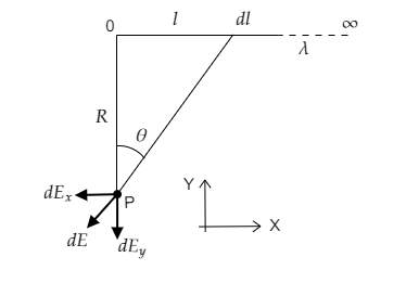
In the above figure, we have a uniform wire of linear charge density $\lambda$ whose length increases infinitely in one direction. The electric field intensity at the point P is to be determined.
For that, we consider a small elemental length $dl$ of charge $dq = \lambda dl$ of the wire at a distance $l$ from its finite end. The point P is at a distance $R$ from the finite end. The electric field vector due to the small element $dE$ at P makes an angle $\theta$. The electric field components due to the small elemental charge $dq$ are given to be $d{E_x}$ and $d{E_y}$.
Step 2: Express the components of the electric field vector at P due to the small elemental charge.
From the figure, we get the distance between the point P and the elemental charge to be $\sqrt {{R^2} + {l^2}}$.
The magnitude of the electric field $dE$ at P due to the elemental charge $dq$ is given by, $dE = \dfrac{1}{{4\pi {\varepsilon _0}}}\left( {\dfrac{{dq}}{{{R^2} + {l^2}}}} \right)$ -------- (1)
Then the components of $dE$ are $d{E_x} = - dE\cos \theta$ and $d{E_y} = - dE\sin \theta$ .
Using equation (1) we get, the x-component of the elemental field intensity,
$d{E_x} = \dfrac{{ - \cos \theta }}{{4\pi {\varepsilon _0}}}\left( {\dfrac{{dq}}{{{R^2} + {l^2}}}} \right)$ ----- (2)
and the y-component of the elemental field intensity, $d{E_y} = \dfrac{{ - \sin \theta }}{{4\pi {\varepsilon _0}}}\left( {\dfrac{{dq}}{{{R^2} + {l^2}}}} \right)$ ------ (3)
From the figure we have $\cos \theta = \dfrac{R}{{\sqrt {{R^2} + {l^2}} }}$ and $\sin \theta = \dfrac{l}{{\sqrt {{R^2} + {l^2}} }}$
Then substitute for $\cos \theta = \dfrac{R}{{\sqrt {{R^2} + {l^2}} }}$, $\sin \theta = \dfrac{l}{{\sqrt {{R^2} + {l^2}} }}$ and $dq = \lambda dl$ in equations (2) and (3).
We then have, $d{E_x} = \dfrac{{ - R}}{{4\pi {\varepsilon _0}}}\left( {\dfrac{{\lambda dl}}{{{{\left( {{R^2} + {l^2}} \right)}^{3/2}}}}} \right)$ ----- (4) and $d{E_y} = \dfrac{{ - l}}{{4\pi {\varepsilon _0}}}\left( {\dfrac{{\lambda dl}}{{{{\left( {{R^2} + {l^2}} \right)}^{3/2}}}}} \right)$ ------ (5)
Integrate both equations (4) and (5) to obtain the electric field intensity at P due to the entire charge.
i.e., integrating equation (4) we have ${E_x} = \int\limits_0^\infty {\dfrac{{ - R}}{{4\pi {\varepsilon _0}}}\left( {\dfrac{{\lambda dl}}{{{{\left( {{R^2} + {l^2}} \right)}^{3/2}}}}} \right)} = \dfrac{{ - \lambda R}}{{4\pi {\varepsilon _0}}}\int\limits_0^\infty {{{\left( {{R^2} + {l^2}} \right)}^{ - 3/2}}} dl$
$\Rightarrow {E_x} = \dfrac{{ - \lambda }}{{4\pi {\varepsilon _0}R}}$
Integrating equation (5) we have ${E_y} = \int\limits_0^\infty {\dfrac{{ - R}}{{4\pi {\varepsilon _0}}}\left( {\dfrac{{\lambda dl}}{{{{\left( {{R^2} + {l^2}} \right)}^{3/2}}}}} \right)} = \dfrac{{ - \lambda R}}{{4\pi {\varepsilon _0}}}\int\limits_0^\infty {\dfrac{{ldl}}{{{{\left( {{R^2} + {l^2}} \right)}^{3/2}}}}}$
$\Rightarrow {E_y} = \dfrac{{ - \lambda }}{{4\pi {\varepsilon _0}R}}$
Step 3: Use the components of the field intensity to find the magnitude of the electric field intensity at P.
The magnitude of the field intensity is given by, $E = \sqrt {{{\left( {{E_x}} \right)}^2} + {{\left( {{E_y}} \right)}^2}}$ -------- (6)
Substituting for ${E_x} = {E_y} = \dfrac{{ - \lambda }}{{4\pi {\varepsilon _0}R}}$ in equation (6) we get, $E = \sqrt {{{\left( {\dfrac{{ - \lambda }}{{4\pi {\varepsilon _0}R}}} \right)}^2} + {{\left( {\dfrac{{ - \lambda }}{{4\pi {\varepsilon _0}R}}} \right)}^2}} = \sqrt {\dfrac{{2{\lambda ^2}}}{{16{\pi ^2}{\varepsilon _0}^2{R^2}}}}$
$\Rightarrow E = \dfrac{\lambda }{{2\sqrt 2 \pi {\varepsilon _0}R}}$
The direction of the electric field is given by, $\tan \theta = \dfrac{{{E_x}}}{{{E_y}}} = 1$
$\Rightarrow \theta = 45^\circ$ .
Thus the magnitude of the electric field intensity at P is $E = \dfrac{\lambda }{{2\sqrt 2 \pi {\varepsilon _0}R}}$ and is directed at $\theta = 45^\circ$.

Note: It is mentioned that the uniform wire is semi-infinite i.e., it extends to infinity at one end. So we integrate equations (4) and (5) from $0$ to $\infty$. Also, it is given that the point P lies perpendicularly to the uniform wire at its finite end. So the electric field vector, the length $l$ and the distance $R$ form the sides of a right-angled triangle and we use Pythagoras theorem to determine the distance between the point P and the small element as $\sqrt {{R^2} + {l^2}}$ .