Question

Draw a curve for showing variation in alternating current with frequency in LCR resonant circuit. Hence obtain an expression of bandwidth.

Answer 1

In a LCR circuit, when the value of capacitive reactance is equal to the inductor reactance and impedance is equal to resistance the value of current increases suddenly. Current takes its root mean squared value at two values of frequency, these values of frequency are known as half power frequency. The bandwidth is the difference between the values of half power frequency.

Complete step-by-step solution:
An LCR circuit is a circuit which contains a resistor, capacitor as well as an inductor. At a certain frequency, the impedance becomes minimum and the current becomes maximum, this condition is called resonance and the frequency is called resonant frequency.

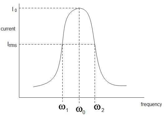
${{\omega }_{0}}$ is the resonant frequency
${{I}_{rms}}$ is the root mean square current

At resonance,
${{X}_{L}}={{X}_{C}}$
We know that,
$\dfrac{{{V}_{0}}}{Z}=I$ - (1)
Here,
${{V}_{0}}$ is the potential difference
$I$ is the current
$Z$ is the impedance

At resonance, $Z=R$ substitute in eq (1), we get,
$\dfrac{{{V}_{0}}}{R}={{I}_{0}}$
$\Rightarrow {{V}_{0}}={{I}_{0}}R$ - (2)
Here,
${{I}_{0}}$ is the maximum current
$R$ is the resistance

When $I=\dfrac{{{I}_{0}}}{\sqrt{2}}$ , the frequency is half power frequency ${{\omega }_{1}},\,{{\omega }_{2}}$ substitute in eq (1), we get,
$\dfrac{{{V}_{0}}}{Z}=\dfrac{{{I}_{0}}}{\sqrt{2}}$

When we substitute eq (2) in the above equation, we get,
$\begin{aligned} & \dfrac{{{I}_{0}}R}{Z}=\dfrac{{{I}_{0}}}{\sqrt{2}} \\\ & \Rightarrow Z=\sqrt{2}R \\\ & \Rightarrow \sqrt{{{R}^{2}}+{{\left( (\omega L)-\dfrac{1}{(\omega C)} \right)}^{2}}}=\sqrt{2}R \\\ & \Rightarrow {{R}^{2}}+{{\left( (\omega L)-\dfrac{1}{(\omega C)} \right)}^{2}}=2{{R}^{2}} \\\ & \Rightarrow {{\left( (\omega L)-\dfrac{1}{(\omega C)} \right)}^{2}}={{R}^{2}} \\\ \end{aligned}$

Substituting, $\omega ={{\omega }_{0}}+\Delta \omega$ in the above equation, we get,
$\Rightarrow {{\left( {{\omega }_{0}}L\left( 1+\dfrac{\Delta \omega }{{{\omega }_{0}}} \right)-\dfrac{1}{\omega _{0}^{{}}C\left( 1+\dfrac{\Delta \omega }{{{\omega }_{0}}} \right)} \right)}^{2}}={{R}^{2}}$

The condition of resonance is,
$\begin{aligned} & {{\omega }_{0}}L=\dfrac{1}{{{\omega }_{0}}C} \\\ & \therefore C=\dfrac{1}{\omega _{0}^{2}L} \\\ \end{aligned}$

When we substitute in above equation, we get,
$\begin{aligned} & \Rightarrow {{\left( {{\omega }_{0}}L\left( 1+\dfrac{\Delta \omega }{{{\omega }_{0}}} \right)-\dfrac{{{\omega }_{0}}L}{\left( 1+\dfrac{\Delta \omega }{{{\omega }_{0}}} \right)} \right)}^{2}}={{R}^{2}} \\\ & \Rightarrow \left( {{\omega }_{0}}L\left( 1+\dfrac{\Delta \omega }{{{\omega }_{0}}} \right)-\dfrac{{{\omega }_{0}}L}{\left( 1+\dfrac{\Delta \omega }{{{\omega }_{0}}} \right)} \right)=R \\\ & \Rightarrow \left( {{\omega }_{0}}L\left( 1+\dfrac{\Delta \omega }{{{\omega }_{0}}} \right)-{{\omega }_{0}}L{{\left( 1+\dfrac{\Delta \omega }{{{\omega }_{0}}} \right)}^{-1}} \right)=R \\\ \end{aligned}$

Applying rules of exponents, we get,
$\begin{aligned} & \Rightarrow \left( {{\omega }_{0}}L\left( 1+\dfrac{\Delta \omega }{{{\omega }_{0}}} \right)-{{\omega }_{0}}L{{\left( 1+\dfrac{\Delta \omega }{{{\omega }_{0}}} \right)}^{-1}} \right)=R \\\ & \Rightarrow \left( {{\omega }_{0}}L\left( 1+\dfrac{\Delta \omega }{{{\omega }_{0}}} \right)-{{\omega }_{0}}L\left( 1-\dfrac{\Delta \omega }{{{\omega }_{0}}} \right) \right)=R \\\ & \Rightarrow 2{{\omega }_{0}}L\dfrac{\Delta \omega }{{{\omega }_{0}}}=R \\\ & \therefore \Delta \omega =\dfrac{R}{2L} \\\ \end{aligned}$

For bandwidth,
$\begin{aligned} & {{\omega }_{2}}-{{\omega }_{1}}=({{\omega }_{0}}+\Delta \omega )-({{\omega }_{0}}-\Delta \omega ) \\\ & \therefore {{\omega }_{2}}-{{\omega }_{1}}=2\Delta \omega \\\ \end{aligned}$

Here, ${{\omega }_{2}}-{{\omega }_{1}}$ is the bandwidth.
Therefore,
$\begin{aligned} & {{\omega }_{2}}-{{\omega }_{1}}=2\Delta \omega \\\ & \Rightarrow {{\omega }_{2}}-{{\omega }_{1}}=2\times \dfrac{R}{2L} \\\ & \therefore {{\omega }_{2}}-{{\omega }_{1}}=\dfrac{R}{L} \\\ \end{aligned}$

Therefore, the bandwidth is $\dfrac{R}{L}$.

Note:
At resonance, the current increases infinitely as the impedance becomes minimum. Half power frequencies are those frequencies at which the current attains its root mean squared value. Root mean squared current is defined as the maximum current divided by root two. It is also calculated by taking the average square of all currents.