Question
Question: An infinite line charge of uniform electric charge density \( \lambda \) lies along the axis electri...
An infinite line charge of uniform electric charge density λ lies along the axis electrically conducting an infinite cylindrical shell of the radius R . At time t=0 , the space in the cylinder is filled with a material of permittivity ε and electrical conductivity σ . The electrical conduction in the material follows Ohm's law. Which one of the following best describes the subsequent variation of the magnitude of current density j(t) at any point in the material?
(A) 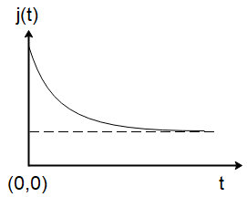
(B) 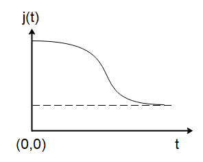
(C) 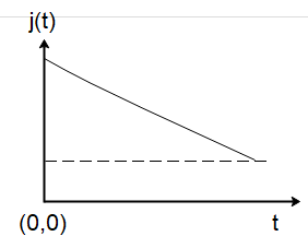
(D) 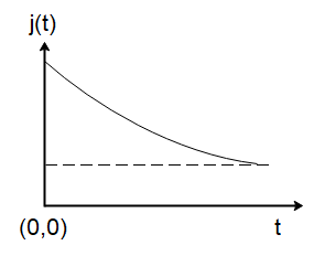
Solution
Hint : In this solution, we will determine the electric field due to a line charge at a distance equal to the radius of the cylinder. The current density generated in the cylinder will be determined using ohm’s law. The current in the
Formula used: In this solution, we will use the following formula:
-Electric field due to a line charge: E=r2kλ where λ is the line charge density of the line charge and r Is the distance of the point from the charge.
- Ohm’s law: J=σE where J is the current density and σ is the electrical conductivity and E is the electric field.
Complete step by step answer
Let us start by calculating the current density in the cylinder. Since the electric field due to a line charge inside the cylinder will be
E=r2kλ ,
We can determine the charge density as
J=σ(r2kλ)
Now we know that the current density is the ratio of the current in the circuit I to the area of the cylinder A . So we can write
J=AI
⇒I=JA
Substituting the value of current density this in the above equation, we get
I=σA(r2kλ)
Since I=dtdq , we can write
dtdq=σA(r2kλ)
The charge in the line charge can be calculated as the product of line charge density and the length as
q=λl
So, we can write
dtd(λl)=σ2πrl(2πε0r2kλ) (∵A=2πrlandk = 4πε01)
Now the length of the line remains constant so the variable in the above equation must be the line charge density which varies with time.
Integrating the above equation with time, we get
λ=λ0e−σt/ε where λ0 is the term containing all the constants.
Multiplying both sides by rσ2k , we get
J=J0e−σt/ε
Hence the graph of current density with time is exponentially decaying with time which corresponds to option (A).
Note
In this solution, it is difficult to confer that the line charge density will vary with time which is why we solve the equations to see that the current density could be varying with time only the line charge density is changing. We must also be aware of the general behaviour of different functions when plotted with respect to time.