Question

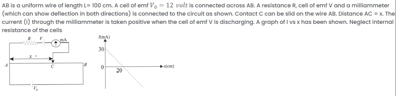
AB is a uniform wire of length L= 100 cm. A cell of emf $V_0$ = 12 volt is connected across AB. A resistance R, cell of emf V and a milliammeter (which can show deflection in both directions) is connected to the circuit as shown. Contact C can be slid on the wire AB. Distance AC = x. The current (I) through the milliammeter is taken positive when the cell of emf V is discharging. A graph of I vs x has been shown. Neglect internal resistance of the cells

Answer 1

V = 2.4 V, R = 80 Ω

Answer 2

To solve this problem, we need to analyze the potentiometer circuit and the given graph of current (I) versus distance (x).

1. Calculate the potential gradient of the potentiometer wire: The length of the uniform wire AB is $L = 100 \text{ cm}$. The cell connected across AB has an EMF $V_0 = 12 \text{ V}$. The potential gradient ($\phi$) along the wire is given by: $\phi = \frac{V_0}{L} = \frac{12 \text{ V}}{100 \text{ cm}} = 0.12 \text{ V/cm}$

2. Formulate the equation for current (I) in the secondary circuit: The secondary circuit consists of a resistance R, a cell of EMF V, and a milliammeter connected between point A and contact C. The distance AC is x. The potential difference across the segment AC of the potentiometer wire is $V_{AC} = \phi \cdot x$. Let's apply Kirchhoff's Voltage Law (KVL) to the loop formed by the resistance R, cell V, milliammeter, and the wire segment AC. The problem states that current I is taken positive when the cell of EMF V is discharging. This means current flows out of the positive terminal of cell V. From the circuit diagram, the positive terminal of cell V is connected towards the milliammeter and then to point C. The current then flows from C to A through the potentiometer wire, and from A, it flows through resistance R to the negative terminal of cell V. Let's assume the potential at point A is 0 V ($V_A = 0$). Then the potential at point C is $V_C = V_{AC} = \phi x$. Applying KVL by moving from A through R, cell V, milliammeter, to C and back to A: Starting from A, moving in the direction of current I (A to R, then to V-, then to V+, then to mA, then to C, then to A): $V_A - I \cdot R + V - V_C = 0$ (Here, $-IR$ is the potential drop across R, $+V$ is the potential rise across the cell V, and $-V_C$ is the potential drop from C to A, as we are moving from C to A along the wire to complete the loop from point A) Substituting $V_A = 0$ and $V_C = \phi x$: $0 - I \cdot R + V - \phi x = 0$ $V - \phi x = I \cdot R$ $I = \frac{V - \phi x}{R}$

3. Use the given graph to find V and R: The graph shows I (in mA) versus x (in cm). It is a straight line, which is consistent with our linear equation for I. The equation $I = \frac{V}{R} - \frac{\phi}{R} x$ is in the form $y = c + mx$, where $c = \frac{V}{R}$ (y-intercept) and $m = -\frac{\phi}{R}$ (slope).

From the graph:

• At x = 0 cm, I = 30 mA. Substituting these values into the current equation: $30 \times 10^{-3} \text{ A} = \frac{V - \phi (0)}{R}$ $30 \times 10^{-3} = \frac{V}{R}$ (Equation 1)

• At I = 0 mA, x = 20 cm (this is the null point). Substituting these values into the current equation: $0 = \frac{V - \phi (20 \text{ cm})}{R}$ Since R cannot be zero, the numerator must be zero: $V - \phi (20) = 0$ $V = 20 \phi$ (Equation 2)

4. Calculate the values of V and R: Substitute the value of $\phi$ into Equation 2: $V = 20 \text{ cm} \times 0.12 \text{ V/cm} = 2.4 \text{ V}$

Now, substitute the value of V into Equation 1: $30 \times 10^{-3} = \frac{2.4 \text{ V}}{R}$ $R = \frac{2.4 \text{ V}}{30 \times 10^{-3} \text{ A}} = \frac{2.4}{0.03} \ \Omega = \frac{240}{3} \ \Omega = 80 \ \Omega$

5. Verification (optional): The slope of the graph is $m = \frac{\Delta I}{\Delta x} = \frac{0 - 30 \times 10^{-3} \text{ A}}{20 \text{ cm} - 0 \text{ cm}} = \frac{-30 \times 10^{-3}}{20} \text{ A/cm} = -1.5 \times 10^{-3} \text{ A/cm}$. From our equation, the theoretical slope is $m = -\frac{\phi}{R} = -\frac{0.12 \text{ V/cm}}{80 \ \Omega} = -\frac{0.12}{80} \text{ A/cm} = -0.0015 \text{ A/cm} = -1.5 \times 10^{-3} \text{ A/cm}$. The calculated values are consistent with the graph.

The values of V and R are 2.4 V and 80 $\Omega$ respectively.